Production Cost Functions and Competitive Markets
Lecture 5

Output and Costs in the Short Run

1. Short run - a period of time so short that at least one factor of production is fixed, usually the physical capital, like structures, machines, and equipment.

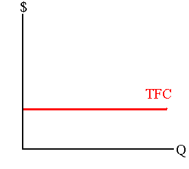
• Total Fixed Costs (TFC) - the costs do not change when production level changes
  • Insurance premiums
  • Property taxes
  • Overhead from administration
  • Bank loans
  • Airlines, hotels, and theme parks have high fixed costs
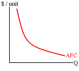
• Average Fixed Costs (AFC) - fixed costs per good produced
  • As production level increases, AFC will get smaller and smaller
  • "Spreading the overhead"
  • The fixed costs is spread out over more units

AFC = TFC / Output

Total Fixed Cost	Average Fixed Cost
Costs	Per-Unit Costs
Output/Quantity	Output/Quantity

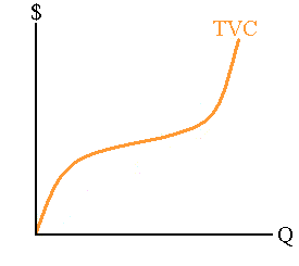
• Total Variable Costs (TVC) - the costs that varies when the production level changes.
  • Labor costs
  • Raw material costs
  • Energy costs such as electricity, water, etc.
  • Labor is a large cost for many tourist related companies
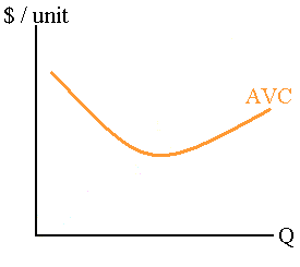
• Average Variable Cost (AVC) - variable costs per unit of a good produced

AVC = TVC / Output

Total Variable Costs	Average Variable Costs
Costs	Per-Unit Costs

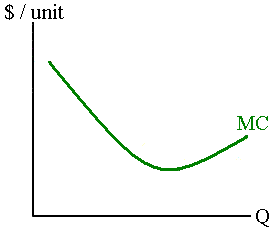
2. Marginal Cost (MC) - the increase in cost as production increases by one unit.

• MC will decline initially, reach a minimum, and then rise
• Example: A hotel starts with 0 workers
• Specialization of labor
  • Production gains
  • MC decreases
    • 1 worker - output is to service 10 rooms (10 rooms per worker)
    • 2 workers - output is to service 30 rooms (15 rooms per worker)
    • 3 workers - output is to service 60 rooms (20 rooms per worker)
• Law of Diminishing Returns
  • Output increases by a smaller and smaller amount as more labor (variable resource) is added to a fixed resource
  • Production inefficiency
  • Exists only in the short run
  • MC increases
    • 50 workers - output is to service 1,000 rooms (20 rooms per worker)
    • 51 workers - output is to service 1,100 rooms (18.3 rooms per worker)

Marginal Cost
Cost per unit
Output/Quantity

3. The Total Costs and Average Curves.

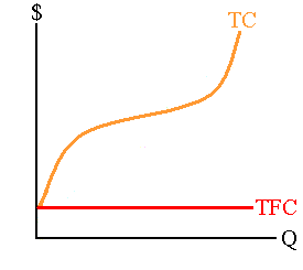
Total Cost (TC) = Total Fixed Cost + Total Variable Cost

TC = TFC + TVC

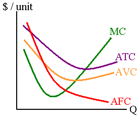
Average Total Cost (ATC) = Average Fixed Cost + Average Variable Cost.

ATC = AFC + AVC = TC / Output

• Relationship between marginal cost and total variable costs
  • MC < ATC, then ATC is decreasing
  • MC > ATC. then ATC is increasing
  • MC intersects ATC at its minimum point
  • Example: Student's score is 80% and student took 2 tests
    • 3rd test (i.e. marginal)
    • Scores 90%, average increases
    • Scores 70%, average decreases

Total Cost Curves	Average Cost Curves
Total cost	Per-unit cost
Output/Quantity	Output/Quantity

Output and Costs in the Long Run

1. Long run - is a period of time sufficient for the firm to alter all factors of production.

• Firms can enter and exit the industry.
• Long run differs by industry.
  • Examples: Long run for an automobile factory using lots of machines may be 7 years.
  • The long run for an internet company may be 1 year.
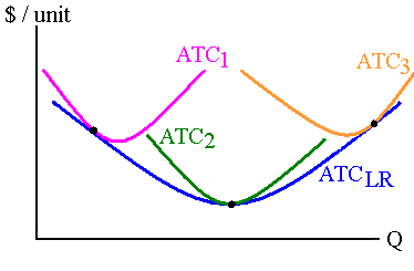
• Long-Run ATC - shows the minimum average cost of producing each output level when a firm is able to vary all production resources, including factory size.
  • Allow the firm to vary among 3 factory sizes: ATC ₁ , ATC ₂, ATC ₃ . Which factory size should the firm produce at?

Long Run ATC
Per-Unit Cost
Output

ATC 2 will give the factory the lowest per unit costs in the long run. The firm will be able to recuperate all its total costs, when: Market price (P*) > = minimum of long-run ATC

2. Why unit costs differ in the long run.

Long Run ATC
Per-Unit Cost
Output

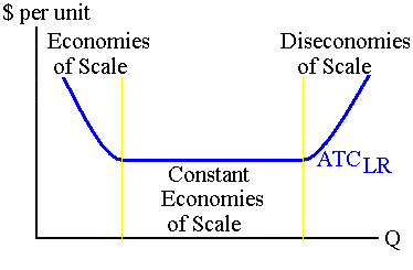
• Economies of scale - per-unit costs fall as output (plant size) expands
  • Financial - a larger firm has access to more financing options
  • Buying and selling - a larger firm can buy or sell in bulk, which leads to discounts
  • Mass production - large amounts of capital and machines
  • Specialization of labor - adding more labor allows workers to specialize in task that they are good at
  • Management specialization - people specialize in finance, personnel, and marketing
  • Technical specialization - a larger firm can use more expensive technology
  • Risk bearing - a larger firm can weather set backs
    • Has diversified business
    • Has more resources
  • Concentration of competitors at tourist destination
    • Competitor's advertising attracts tourists to the area
  • Examples
    • Automobile
    • Electricity
    • Natural gas
    • Telecommunications including internet services
    • Computer chips
• Constant returns to scale - per-unit costs are constant as plant size is changed.
  • Small firms can be just as efficient as large firms.
    • Apparel
    • Food processing
    • Publishing
    • Lumber
    • Retailing
    • Wood products
• Diseconomies of scale - per-unit costs rises as output (plant size) expands
  • Bureaucratic inefficiencies
  • More difficult to coordinate and manage workers
  • Monitoring and over site problems
  • Tourist destination - overcrowding and congestion

3. Firms become larger through mergers

• Merger - firm takes over and integrates another firm
• Horizontal integration - firm takes over another firm in the same market
  • Example - one hotel chain takes over another hotel company
  • Economies of scale
  • Reduce advertising
  • Adjust discounts to maximize profits
  • If one company owns all the hotels in one area, then it may have monopoly power
• Vertical integration - a firm takes over another firm in the supply chain
  • An airline company that services a tourist destination buys a hotel chain there
  • Company may have a cost advantage
  • Gives control over the supply, and hence the quality level
  • Note - many energy companies are vertically integrated
    • Petroleum company extracts, refines, and sells fossil fuels to consumers
• Conglomerate - a firm takes over other firms in different, unrelated markets
  • Diversify its products and services, and reduce risks
  • Firm may leave a dying market and enter a new market
  • Example - Carlson Company
    • Hotels
    • Restaurants
    • Travel agencies
    • Marketing consultant agencies

Pure Competition

1. Purely Competitive Firms - accepts the market price in order to sell their products. They are also called price takers
   • Characteristics:
     • All firms produce an identical product
       • Consumers do not care where they buy the product
     • A large number of firms are in the market
     • Each firm supplies only a small portion of the total supplied to the market
       • One firm cannot influence the price of the market
     • No barriers to entry or exit exist
       • Example: If one firm earns economic profit, then rival firms can easily enter the market and try to earn profits
     • The firms maximize profit by adjusting production level, but cannot influence market price.
2. Examples
   • Agricultural markets are competitive
   • International tourist destinations can be very competitive

Output in the Short Run

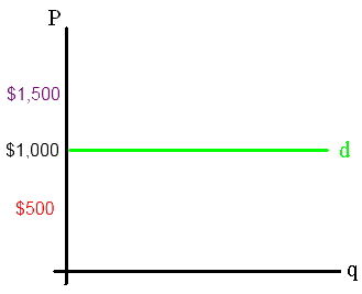
1. Marginal Revenue (MR) - is the change in total revenue when output increases by one unit.

• A tour company sells airline-hotel packages at the market price
• Refer to the graph below
  • If the company sells one more package, it receives $1,000 (MR). If the company sells another package, it receives another $1,000 (MR).
  • If the company raises its package above the market price, then tourists do no buy it.
    • Tourists buy the package from competitors for $1,000
  • If the company sells his package below the market price, then it receives lower revenue (loses money)
  • Thus, it sells all of its packages at the market price, so MR = P* = $1,000.

Price Taker's Demand Curve
A Tour Company	The Market
Price	Price
Quantity	Quantity

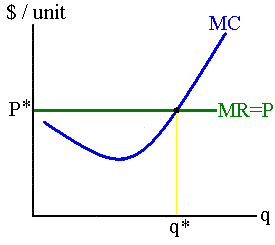
2. Profit maximization - the price taker will expand output in the short run until:

P* = MR = MC

Note: The market price is P* and marginal cost is MC. Further, the MR = MC maximizes profits for monopolies, oligopolies, and monopolistically competitive firms, while MR = P* is only valid for price takers.

	This rule maximize the firm's profits (or minimize its losses)
	Example: If MR = $3 and MC = $2. MR > MC, the firm will collect $3 for selling that last "additional" unit that only costs $2 to produce. Profit increases by $1. If MR = $3 and MC = $5. MR < MC, the firm will collect $3 for selling that last unit that costs $5 to produce. The firm should reduce production by 1 unit to increase profits.

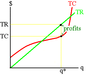
• Price takers earn profits by maximizing total revenue (TR) and minimizing total costs(TC)
  • Total Revenue (TR) = P * q
  • Profits = TR - TC
  • Taking vertical slices (adjusting output q) until TR -TC is maximized, which is shown below:

Firm
$

The point where profit is maximized is at the production level q when MC = MR = P*

Firm
Price / Per-unit costs
Quantity

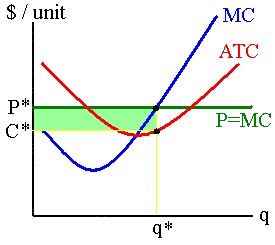
• Using the marginal cost, market price, and average total cost, we can show a competitive firm earning a profit.
  • Firm earns a profit when Market Price > ATC
  • The "green" rectangle is firm's profit
• The derivation is:

Profit = Total Revenue - Total Cost

Profit = P q - ATC q = (P - ATC) q

Firm
Price / Per-unit costs
Quantity

3. Losses and going out of business.

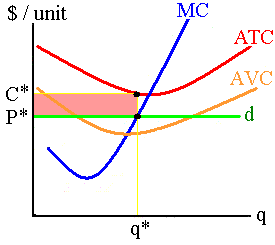
• Firm produces quantity q where MC = MR = P
  • ATC > Market Price, the firm is earning a loss, or profit is negative .
  • Profit = Total Revenue - Total Cost
  • Profit = P q - ATC q = (P - ATC) q
  • The loss = "The red area"

Firm
Price / Per-unit costs
Quantity

• Short-run.
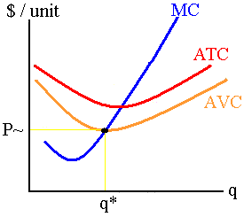
  • A firm will operate in the short run with losses, if it can cover its average variable costs.
  • Example: Hotel Room
    • AVC = $20 per room (labor), AFC = $10 (bank loan)
    • The hotel market is competitive, so P* = MR = MC
      • If P* = $15; firm cannot cover its variable costs, so it shuts down; it still pays its fixed costs
      • If P* = $20; firm covers its variable costs, but earns a loss
      • If P* = $25; firm still earns a loss, but also covers some of its fixed costs
      • If P* = $30; firm breaks even
      • If P* > $30; firm earns an economic profit
  • Shutdown - temporary halt in the production or operation of a business.
    • A firm shuts down when P* < AVC
    • The firm still pays fixed costs during the shutdown.
    • Motels, restaurants, and theme parks shutdown during off seasons
• Long-run.
  • A firm will "go out of business" in the long run, if P < ATC.
  • Going out of business - firm permanently exits the market and avoids paying fixed costs
  • Example - art galleries have high fixed costs
    • During a recession, customer demands quickly drop
    • Thus, art galleries go out of business

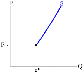
4. A competitive firm maximizes profits when it produces at P* = MC.

• A firm's short-run supply curve is its marginal cost curve above average variable cost.
• Firm produces if the market price exceeds its average variable costs.
• Law of Supply - as the price of a product increases, firms will increase quantity supplied.

A Firm's Cost Curves	A Firm's Supply Curves
Price / Per-unit costs	Price / Per-unit costs
Quantity	Quantity

Output Adjustments in the Long Run

• In the long-run, firms earn zero economic profit
  • A normal rate of return, i.e. accounting profit
• If P* > ATC, firms earn an economic profit
  • New firms enter the market
  • SR Supply increases while the price decreases until it equals P = ATC
  • Economic profit = 0
• If P* < ATC, firms earn a loss
  • Some firms leave the market
  • SR supply decreases, while the price increases until it equals P = ATC
  • Economic profit = 0
• Long-run equilibrium
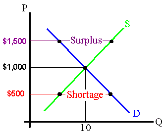
  • The market determines the price and quantity of vacation packages
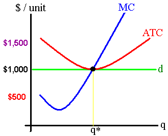
    • P* = $1,000 and market quantity = 10 (thousand)
  • Each firm supplies q quantity of travel packages
    • Earn zero economic profit
    • P* = ATC = $1,000

A Travel Firm's Long-Run Cost Curve	The Travel Package Market
Price / Per-unit costs	Price / Per-unit costs
Quantity	Quantity (in thousands)

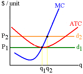
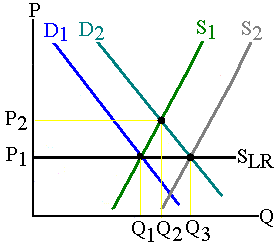
• Example: The incomes in the United States increase
  • Consumers buy more vacation packages (travel is a luxury good)
    • The demand curve shifts right.
      • New market price is P ₂
      • Quantity supplied and sold is Q ₂
  • Firms expand output to q ₂
    • Earn economic profits (P ₂ > ATC)
  • Long-run equilibrium
    • New firms enter the travel vacation market
    • Short-run supply increases
    • Price decreases, until P ₁ = ATC again
  • Result:
    • Same market price, P ₁
    • More travel packages are offered and sold, Q ₃
    • More firms are in the market and all earn zero economic profit

A Travel Firm's Long Run Cost Curve	The Travel Vacation Market
Price / Per-unit costs	Price / Per-unit costs
Quantity	Quantity

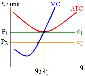
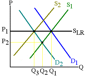
• Economic losses and exit
• Example: Riots in Egypt (tastes and preferences)
  • The original demand & supply curves are D ₁ & S ₁
  • Demand curve shifts left.
    • New market price is P ₂
    • Quantity supplied and sold is Q ₂
  • Firms contract output to q ₂
    • Earn economic losses (P ₂ < ATC)
  • Long-run equilibrium
    • Some firms leave the hotel market
    • Short-run supply decreases
    • Price increases, until P ₁ = ATC again
  • Result:
    • Same market price, P ₁
    • Less hotel rooms are produced and sold, Q ₃
    • Less firms are in the market and all earn zero economic profit

A Hotel in Egypt	The Hotel Market in Egypt
Price / Per-unit costs	Price / Per-unit costs
Quantity	Quantity

• Long-run supply - the minimum price which firms will supply various production levels when all factors of production can be adjusted.
  • The long-run supply is the black lines in the milk and rice markets
• Constant-cost industry - industry were resource prices remain unchanged as market output is expanded
  • Long-run market supply curve is horizontal (perfectly elastic)
  • Illustrated above in milk and rice markets
  • An expanding/contracting industry has no impact on the resource markets, because it is a small industry

Terminology