Welfare Measures
Lecture 4

Deriving A Marshallian Demand Function

1. A consumer maximizes his utlity given his budget constraint

• Budget constraint - shows how much a consumer can purchase from two goods given his income and product prices
• A consumer's purchases does not affect the market price
  • Many consumers in the market
    
  • Pure competition on demand side of market
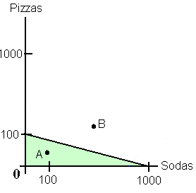
• Example - The easy way
  • A person's income is $1,000
  • Price of pizza is $10
  • Price of soda is $1
• Math:
  • If a consumer spent all his money on pizza, then he can buy 100 pizzas
  • If a consumer spent all his money on sodas, then he can buy 1,000 sodas
  • Budget constraint is shown below

2. A person has a set of prefereneces for pizza and sodas

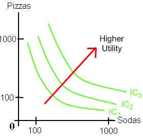
• Indifference curves - shows how much utility a consumer gets from consuming two goods
  • The graph has three sets of preferences
    • Each indifference curve is a level of utility, and shows how much sodas and pizza yield that level of utilty
  • The further right this consumer goes, then the more utlity that person has from pizza and sodas
  • IC ₃ gives higher utility than IC ₂, and IC ₂ gives higher utility than IC ₁

• How do we know preferences have this shape
• Based on Law of Diminishing Marginal Utility
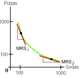
  • Marginal Rate of Substitution (MRS) - the consumer is willing to give up some pizza to get more soda
    • Slope of the tangent line where it touches the indifference give in one spot
  • MRS ₁ - drawing a triangle to indicate the slope of the line
    • Person has lots of pizza but little soda
    • Notice the height of the triangle is greater than the width
    • Person is willing to give up alot of pizza to get a little more soda
  • MRS ₂ - At this point, person has lots of soda but little pizza
    • The triangle has a small height but a large amount of soda
    • For this person to give up a little pizza, you have to get him a lot more sodas (he already has plenty).

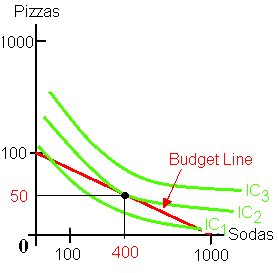
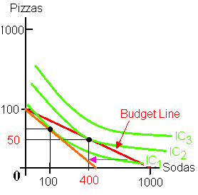
• A consumer's budget line restricts how much goods a consumer can consume
• Looking at the graph below, the consumer wants to maximize utility
  • Assume his income is $1,000 and prices for both pizza and soda is $1
• The highest indifference curve he can attain is IC ₂
  • At that point, he consumes 50 pizzas and 400 sodas

3. Derive a Marshallian Demand

• Assume the price of soda increases from $1 to $2, then budget line shifts inward for sodas
• Consumer will try to obtain highest indifference curve, which is IC ₁
• Consumer's utility is lower, but the price of soda increased, thus he consumes less

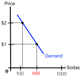
• We can graph the demand for sodas
  • When price of soda is $1, he consumes 400 sodas
  • When price of soda is $2, he consumes 100 sodas
• His demand function for soda is shown below

4. A consumer maximizes his utility given a budget contrraint

In mathematical terms, it is written as

The solution to the problem is:

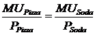
• MU is marginal utility and P is price.
• When you divide by price, you are expressing numbers as "per $1."
• We are removing price differences among all products, so marginal utility can be compared.

If the following condition exists,

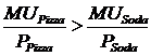
If the consumer had one more dollar, then he would buy pizza, causing the marginal utility for pizza to decrease.

Deriving A Hicksian Demand Function

1. Hicksian Demand function

• Also called a c compensated demand function
  • Utility is held constant
  • Removing the income effect
• Two demand curves
• Hicksian demand curve 1
  • Compensating Variation (CV) - old utility and new prices
  • Using same example as Marshallian demand curve
  • Assume the price of soda increases from $1 to $2, then budget line shifts inward for sodas
  • Income effect - the price of soda is higher, so the consumer's real income fell
    • Give the consumer more money so he ends up on the original indifference curve
  • Hicksian demand only contains the substitution effect
    • The income effect was removed

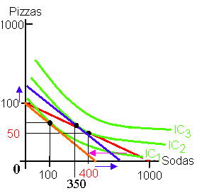
• The consumer ends up on the original utility function
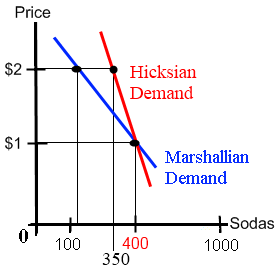
• We can graph the demand for sodas
  • When price of soda is $1, he consumes 400 sodas
  • When price of soda is $2, he consumes 350 sodas
    • Consumer is compensated loss of real income
    • Marshallian demand was 100 sodas
• Both the Marshalliam and Hicksian demand functions for soda are shown below
  • Hicksian demand functions are steeper (for normal goods)
  • Removed the income effect

• Hicksian Demand Curve 2
  • Equilivalent Variation - new utility and old prices
  • Using same example
  • Keep consumer on the new, but lower utilty function
  • If there was no price increase, how much income would the consumer pay to keep the original prices

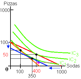
• At new utilty, the price is $1 and the consumer buys 350 sodas
• We would have to select another price and do the same to get a second point
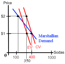
• Equivalent Variation, just shift the Hicksian CV to the left
• All three demand functions are shown

Social Welfare

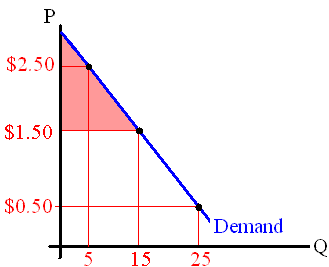
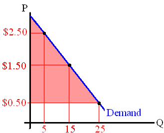
1. Marshallian Consumer Surplus - the area below the demand curve but above the actual price paid.

• Measure of social welfare
• An aggregate benefit to all consumers in the market
• Includes the income effect from a price change
  • Consumers' surplus is approximate
  • The smaller the income effect, the better the approximation
• The market price of coffee is $1.50 and consumers buy 15 (million) pounds of coffee.
  • I place a $2.50 value on this soda, but bought it for $1.50
  • I received a benefit of $1.00
• If the market price of the soda decreases to $0.50, consumers' surplus increases!
  • Social welfare increases

Demand for Coffee	Demand for Coffee
Price	Price
Quantity (in thousands)	Quantity (in thousands)

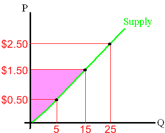
2. Producer Surplus - the area above the supply curve but below the actual sales price.

• Measure of social welfare
• An aggregate benefit to all producers in the market
• Producers' surplus is total fixed costs + profits

Supply of Coffee
Price
Quantity (in thousands)

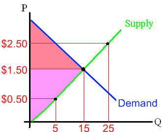
3. Social Welfare is the sum of consumer plus producers' surpluses

Supply of Coffee
Price
Quantity (in thousands)

4. Hicksian Welfare Measures

1. Compensating Variation (old utility, new prices)
   • Price Decrease
     • The income that could be taken away from the consumer to make them as happy as before
   • Price Increase
     • The income that would be given to make the consumer as happy as before the change
2. Equivalent Variation (new utility, old prices)
   • Price Decrease
     • The income that would have to be given to consumer to keep it at the higher price
   • Price Increase
     • The income that the consumer would pay to keep it at the lower price
3. Contingent Evaluation - measure a consumer's preference via survey
   • Usually used in environmental evaluations
   • Example - government plans to expand an airpot at a tourist destination and increases taxes on airline tickets to pay for it.
     • Compensating Variation - how much should the government give the tourists to compensate for the higher price
     • Equivalent Variation - how much would the tourists pay to keep the original airline prices
   • Has problems - consumers are answering hypothetical questions and consumers may be generous in their answers
     • Answers would be different if consumer had to reach into his/her pocket.

Upward Sloping Demand Curves

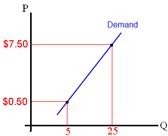
1. Giffen Good - as market price increases, then quantity demanded increases.

• Demand function has a positive slope and elasticity
• Sir Robert Giffen
• Inflicts the poor
  • The staple good must constitute a large portion of the poor's budget
  • The staple has few substitutes
  • As tthe price for a cheap staple increases, the poor cannot afford the better quality food, and buy more of the cheap staple
• The income effect overwhelms the substitution effect
  • A price increases causes a decline in real income
  • Thus, Giffen good has to be inferior
• Examples - staples for the poor
  • Rice
  • Noodles
  • Potatoes

Potatoes Market
Price
Quantity

2. Veblen Good - another positively sloped demand function

• Thorstein Veblen
• Why?
  • Snob Effect - price becomes a measure of quality
  • Bandwagon Effect - preferences for a Veblen good increase, as more consumers buy it
  • Buying the good confers a status symbol
• Example
  • Expensive wines
  • Luxury cars
  • Designer handbags
  • Exotic expensive vacations

Terminology